
Robotics
A Generic Framework for Evaluating LiDAR Performance Across Varying Environments
A blog post introducing a new framework/metrology that can be used to evaluate any Lidar against any medium

September 21, 2026
A blog post introducing a new framework/metrology that can be used to evaluate any Lidar against any medium
Hey, I'm Aarush Jain. During my 8-month internship at Polymath Robotics this year, I worked on building a reusable, scalable framework to test how different LiDARs—with known baseline specs—perform against any environment with exact, measured dimensions.
Building a metrology to evaluate LiDAR performance in a repeatable way is difficult.
At Polymath, we serve many different customers operating across diverse settings and environmental conditions. Because different LiDAR models behave differently under varying conditions, understanding which ones perform best in each scenario helps us determine the right model types for specific projects.
To properly evaluate a LiDAR, we first establish a clear evaluation criteria, followed by a set of specific metrics within each category. Take a look at the categories and metrics we came up with below:
ex. RangeDistributionHealth: How far off its reported distance to each point is, expressed as a percentage.
ex. SpatialDropout: The fraction of the target that never got a single return the entire run (dead spots).ex. RangeConsistency: How much its 3D range reading wobbles frame to frame.ex. NearestNeighbourSpacing: How far apart neighbouring points land (tighter means denser).The core runtime stack of the framework is split into 5 main components with the rest of the modules providing abstractions or utilities:
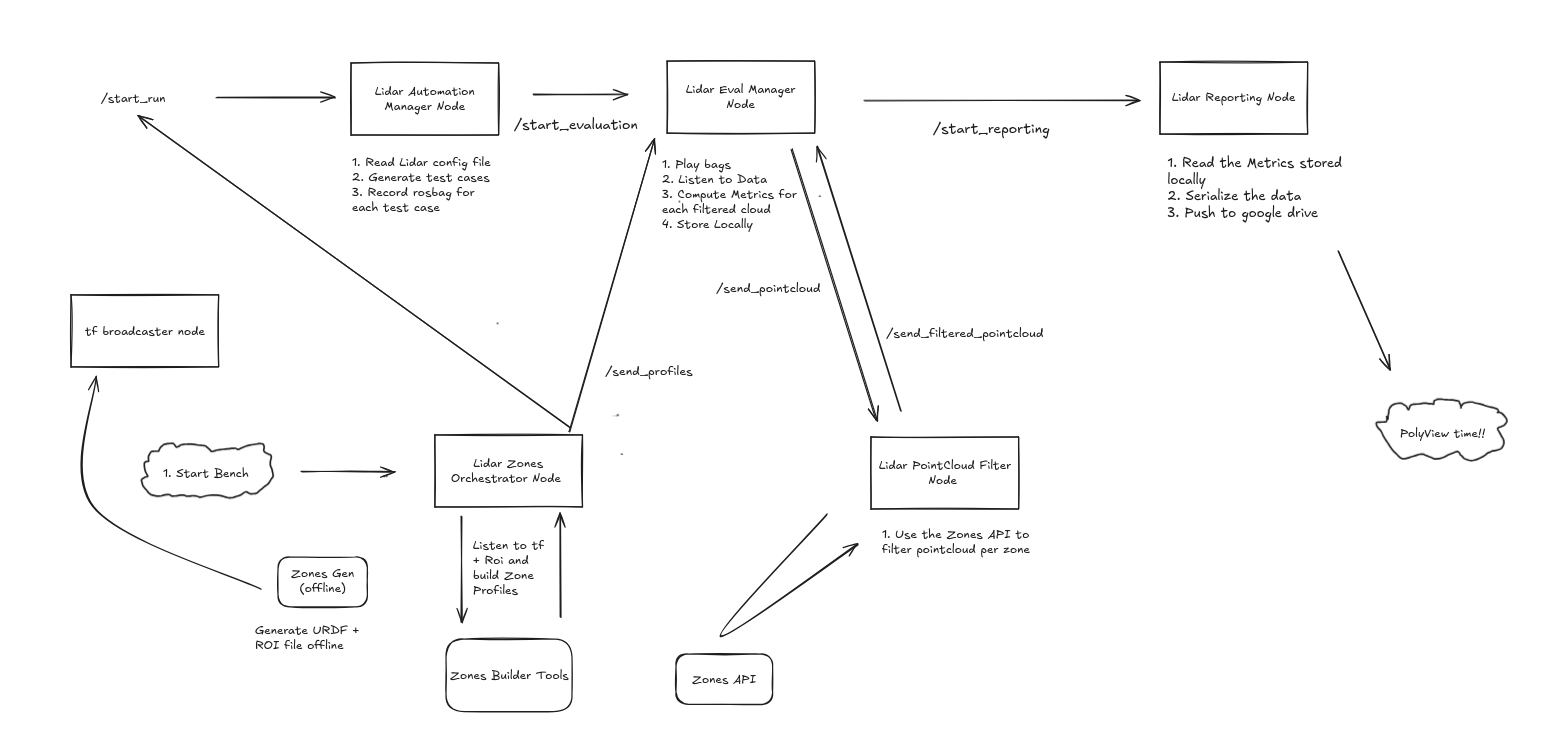
lidar_automation_manager: If you need live rosbag capture, this package automates rosbag data capture for different cases(different parameter values, different panning angles, etc.)lidar_eval_manager: Acts as the core manager of the pipeline and communicates with the rest of the modules to play bags for each case, compute metrics using the metrics library, and reports/pushes to the databaselidar_zones : The central framework for defining different evaluation zone types and their operations plus provides the zones API referenced by all the other components of the stacklidar_pointcloud_filter : Takes in the raw pointcloud per scan + Zones API and returns 2 sets of filtered point clouds for each zone lidar_reporting : Retrieves the metrics computed/stored locally, serializes the data for your chosen database, and pushes the metrics + any visualization data to google drive(or your chosen backend)lidar_metrics_library is where the actual evaluation lives and it’s purely a python library that accepts a sets of zones + the 2 types of filtered pointclouds per zone and computes Lidar metrics per zone that are stored in a yaml file. The library, like the zones framework, was designed to be scalable so that different users can add their own metrics or disable metrics they don’t need with minimal code changes beside the actual metric code.
It involves 4 main components:
class MyMetricPlugin(BaseMetricClass):

    def __init__(self, pointcloud_by_zone, profiles, baseline_profiles):
        # declare your variables
        super().__init__(pointcloud_by_zone, profiles, baseline_profiles)
    def setup(self):
        # One time initialization of vars + anything else needed on startup
    def update(self, pointcloud_by_zone):
        # Called for every PointCloud Message
        # do any processing needed
    def compute():
        # Called at the end of run
# Compute and return the metricComputing lidar metrics is only the first part of the evaluation framework. It’s also very important to know how to present technical results in a nice consumable fashion to an audience who can understand them.
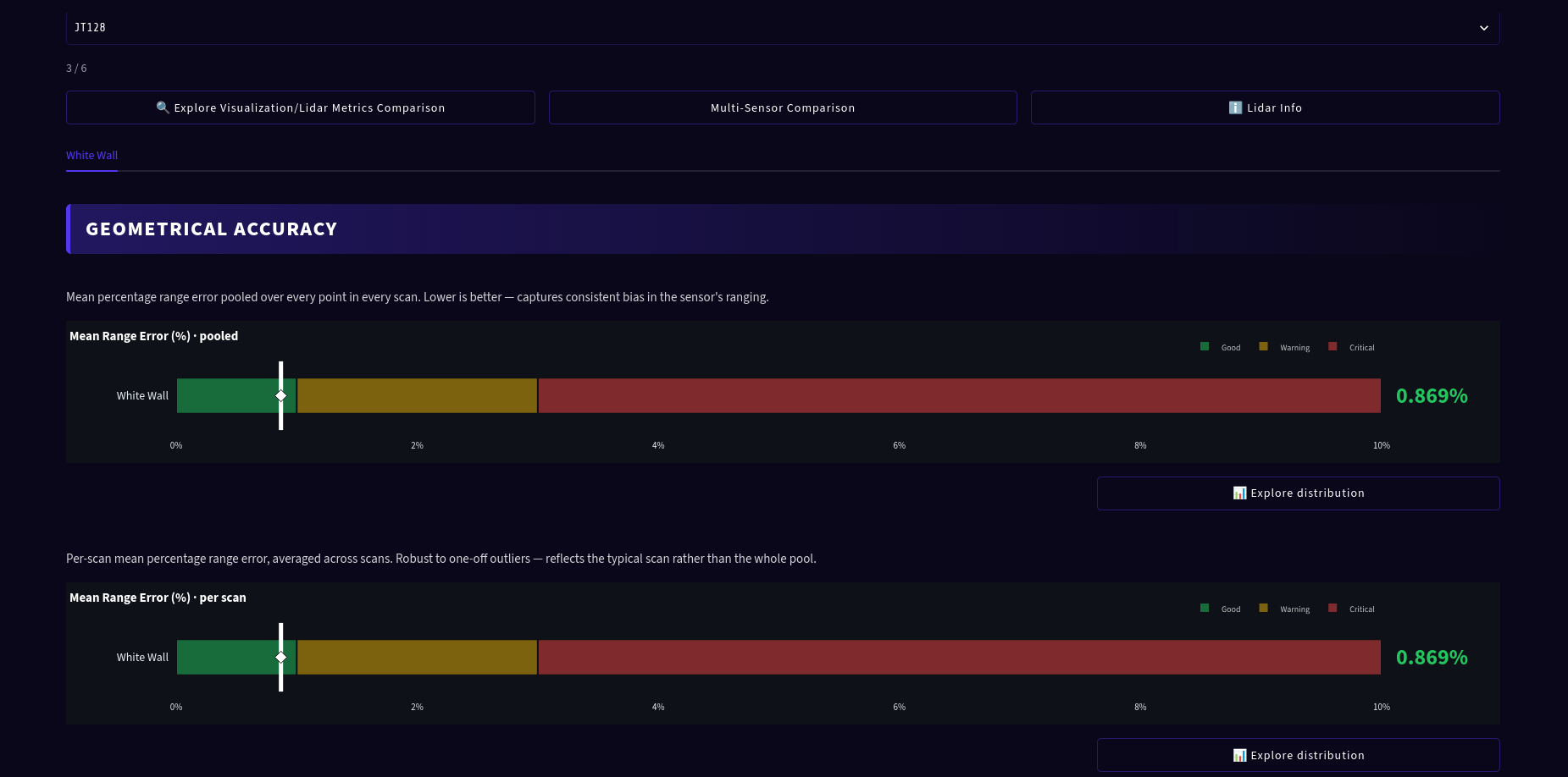
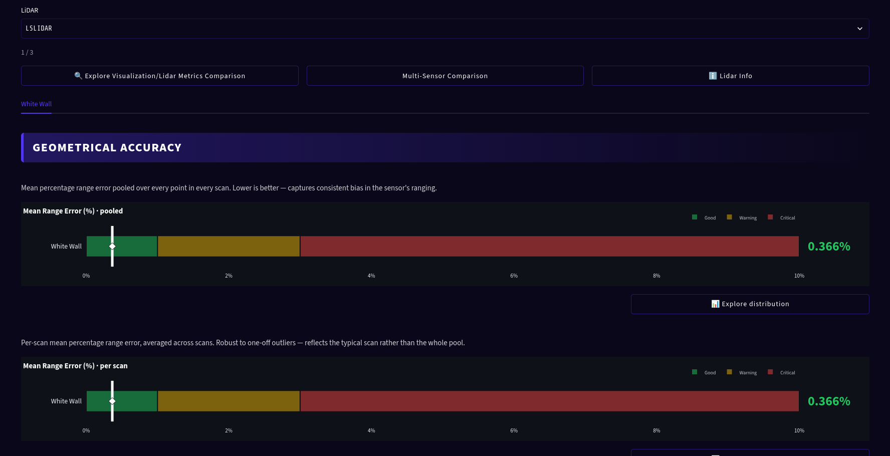
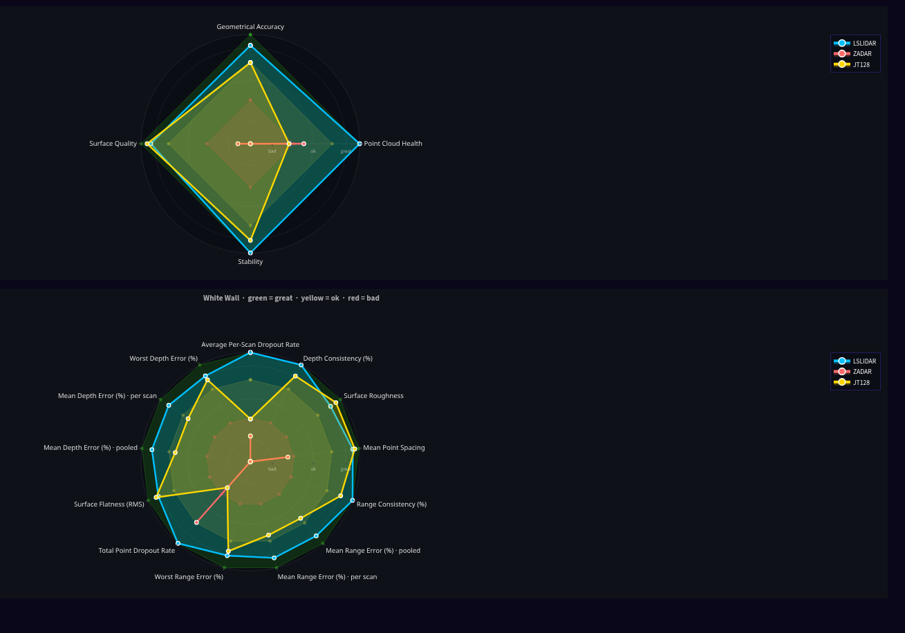
PolyView is an evaluation dashboard built using streamlit that provides the following:
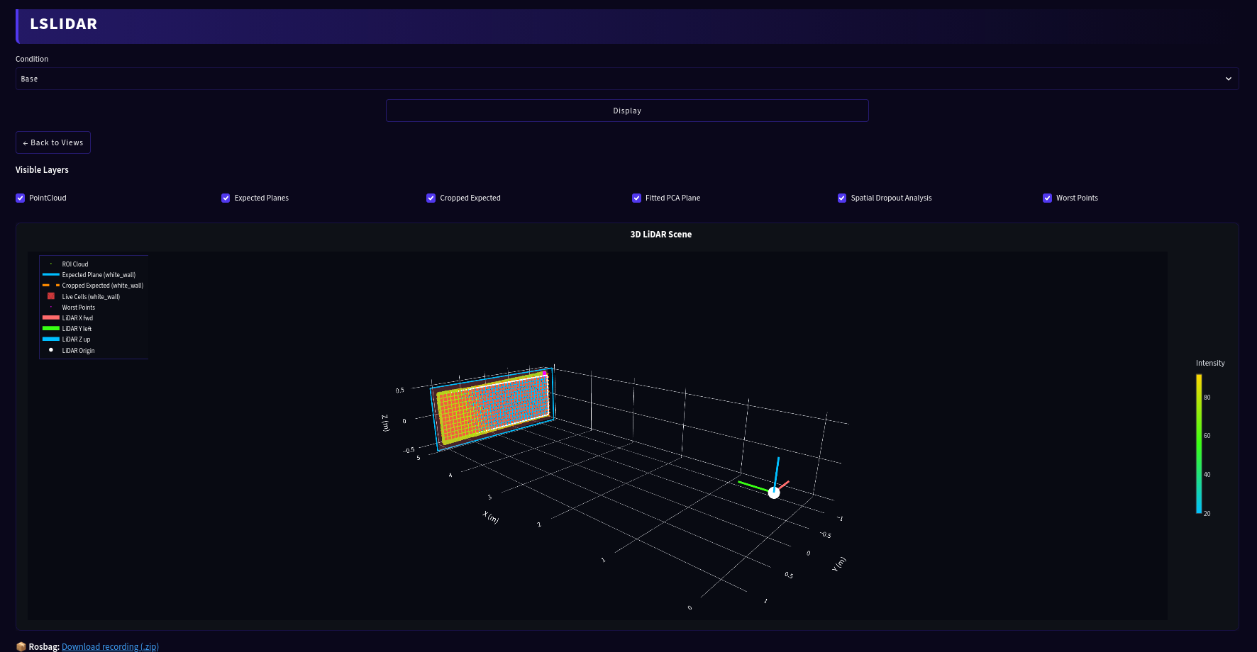
Detailed instructions are available in the public documentation, but you can follow these quick steps after cloning the repository:
Build and run the framework's Docker container immediately after cloning to install all ROS dependencies and internal developer tools.
./run_container.shNow comes the fun part where you get to break your environment down into zones and wire them up in a yaml file.
Writing an environment file is a lot like writing a URDF, except…… much easier. No XML, no <link> soup, no closing tag you forgot about three screens ago. Just plain English and a tape measure.
Say you want to test against a white wall—a planar zone. Start with the basics: the environment's name, where its rosbags get stored, and how long each recording runs. Then list your zones in a steady order under zones. We've only got the one.
name: white_wall_in_front_of_conference_room
bag_recorder_directory: 'CONFERENCE_ROOM_WHITE_WALL'
bag_recording_duration: 20   # seconds per case

zones:
    - "white_wall"

zone_properties:
    white_wall:
        frame: "white_wall"
        type: "planar"
        color: [255, 255, 255]
        height: 1.0287
        length: 2.4638
        z_offset: 0.5588        # how high off the ground the bottom edge sits
        y_padding: 0.101        # trim per side, applied inward
        z_padding: 0.1

world_placement:
    child_zone: "white_wall"
    x_offset: 1.72
y_offset: 0.0zone_joints)One wall is a fine place to start, but real scenes have stuff in them. Here's a whiteboard with a suitcase parked next to it:
name: coop_plus_maiku_hangout
bag_recorder_directory: 'COOP_HANGOUT_BAG'
bag_recording_duration: 20

zones:
    - "whiteboard"
    - "blue_suitcase"

zone_properties:
    whiteboard:
        frame: "whiteboard"
        type: "planar"
        color: [255, 255, 255]
        height: 1.1684
        length: 2.4003
        z_offset: 0.6985
        y_padding: 0.1016
        z_padding: 0.1016

    blue_suitcase:
        frame: "blue_suitcase"
        type: "planar"
        color: [0, 128, 202]
        height: 0.6604
        length: 0.4572
        z_offset: 0.0762
        y_padding: 0.4572
        z_padding: 0.4572

zone_joints:
  whiteboard:
    left_zone:
      zone: blue_suitcase
      x_offset: -0.1524
      y_offset: 0.127

world_placement:
    child_zone: "whiteboard"
    x_offset: 3.81
    y_offset: 0.0
A few things to keep in mind are:
world_placement.child_zone). Every other zone finds its place by hanging off a neighbour, eventually finding its placement from the anchor zoneleft_zone puts the neighbour in +Y, right_zone puts it in −Y. Two sides, no up or down.y_offset: The gap between the two facing edges (NOT THE CENTER) of 2 zones next to each other z_offset from the ground and height.The environment file describes the room. The LiDAR file describes the thing looking at it—and it's why swapping sensors doesn't cost you a line of code.
lidar:
  # ── Identity ──
  frame:               rslidar
  folder:              E1R
  point_cloud_topic:   /rslidar_points

  # ── Mount pose ──
  joint_xyz_m:         [0.0, 0.0, 0.05]
  joint_rpy_rad:       [0.0, 0.0, 0.0]

  # ── Bench geometry ──
  map_to_motor_height_m:   0.9406
  motor_to_lidar_height_m: 0.0889

  # ── Driver ──
  ros2_driver:         rslidar_sdk
  driver_command:      'ros2 run rslidar_sdk rslidar_sdk_node'
  driver_config_file:  '/path/to/rslidar_sdk/config/config.yaml'

  # ── Sweep ──
  angles:              [10.0, -7.0]
  parameter_names:     [min_distance, max_distance]

  # ── Sensor specs ──
  horizontal_fov_deg:        120.0
  vertical_fov_deg:          90.0
  horizontal_resolution_deg: 0.625
  vertical_resolution_deg:   0.625

  # ── Parameters under test ──
  min_distance:
    type:    double
    default: 0.2
    values:  [0.2, 1.0, 5.0]
    path:    lidar.0.driver.min_distance
    description: Minimum range threshold in meters.

  max_distance:
    type:    double
    default: 200.0
    values:  [100.0, 200.0, 500.0]
    path:    lidar.0.driver.max_distance
description: Maximum range threshold in meters.path: Where that parameter lives inside the driver's own config file—that's how the bench pokes it between cases.You've got your environment and LiDAR files written. Now let's point the framework at them.
You can use polysetup - a python CLI tool that sets up your framework to evaluate your chosen Lidars in your properly defined environment. We like just a lot here because it makes our workflows easier so most of the common calls to the tool are wrapped around some easy to use just recipes.
Configuring a run requires just a single recipe:
just setup-ws [environment] [lidar]

# Ex. just setup-ws white_wall_in_front_of_conference_room robosense
source install/setup.bashThe bench runs in one of two modes, which you select prior to configuring.
If you already have bags and want to work without hardware or a live sensor:
just disable-bag-recording
just setup-ws [environment] [lidar]If you have a LiDAR plugged in and want to capture fresh recordings, this brings up lidar_automation_manager, which records a bag per case and kicks off the evaluation automatically:
Bash
just enable-bag-recording
just setup-ws [environment] [lidar]You can also evaluate Lidars with their origins aimed at different panning angles. This way, you get to evaluate the entire field of view and not just a concentrated part which is pretty useful however, you will need to write your own code or package to subscribe to the motor angle topic and properly move your particular bench.
just enable-angle-detection
just setup-ws [environment] [lidar]
Similarly, to disable it, execute:
just disable-angle-detectionWe strongly recommend you use google drive/google sheets as your database just because there’s already code to push and pull everything from here. To successfully wire up a google drive folder/database, you need to create a google cloud account with a secret key and then follow the auth.env.example in lidar_eval_backends to set up your secrets and folder id locally so you’re properly authenticated.
Whether evaluating existing bags or capturing live data, the launch process is identical.
Run the launch command in your main terminal:
just launch-benchWatch the logs for this handshake to confirm the system is ready:
[zones_orchestrator_node] [INFO]: Profiles built successfully — /get_profiles service is ready
[eval_framework_manager_node] [INFO]: BaselineProfiles received: 1 zone(s)Open a second terminal, source the overlay, and trigger the run:
source install/setup.bash
just start-run
start-run automatically adapts to the recording mode you selected in Step 3:
We always welcome contributions that enhance the framework and make life easier for everyone evaluating LiDARs. There are a few ways to pitch in:
At the end of the day, these numbers look cool and all but how do they actually help us? In order to make informed decisions on choosing the right Lidar, we evaluate metrics across 4 different categories (geometrical accuracy, geometrical stability, pointcloud health, and Surface Quality) because they each tell us something different.
For example, at Polymath, we often deploy the Hesai JT128 Lidar model on most of our customer vehicles. Recently, Hesai Technology released a new Patch upgrade that was designed to introduce advanced point cloud processing modes, add Layer 2 PTP time synchronization, improve GPS startup behaviour, and critical bug fixes related to point cloud continuity and hardware stability.
To generate a good baseline, we tested against a white wall and after running the tests, we discovered some very interesting results. The first was that the geometrical accuracy using the projectively cropped point cloud of the new firmware uploaded was slightly better than the accuracy of the model with the old firmware. However, the scan to scan depth consistency was significantly worse for the new firmware compared to the old firmware.
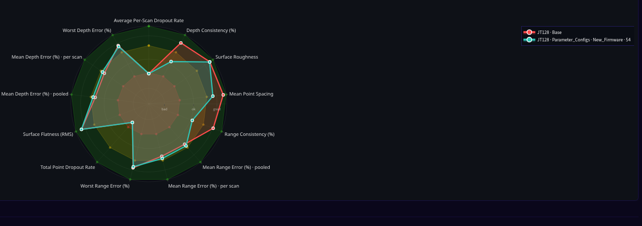
Now, this is where you need to really understand Lidar’s in order to understand the results. Slightly higher accuracy in a controlled setting with no interference coupled with substantially worse consistency frame to frame suggests that the new firmware removes systematic bias from the filtering which increases noise but in exchange, reflects the real world more accurately. Noise is also preferred because we can do our own filtering on top of it without any of the systematic bias skewing the data. An combination of near perfect accuracy coupled with a stability inconsistency is the next best thing a Lidar can give us that’s actually realistic.
And there you have it! Anytime you need to evaluate and cross-compare different lidars against each other, this framework should really help speed things up for you.
If you’re interested in hearing more about the framework and how it works, I will be giving a talk at ROSCon in Toronto this upcoming September. If you’re attending, feel free to check out my talk:
Link to Documentation: https://polymathrobotics.github.io/lidar_eval_framework/docs/intro
Link to Github Repo: https://github.com/polymathrobotics/lidar_eval_framework
Link to Polymath Robotics: https://polymath-lidar-eval-dashboard.streamlit.app/
Hey, I'm Aarush Jain. During my 8-month internship at Polymath Robotics this year, I worked on building a reusable, scalable framework to test how different LiDARs—with known baseline specs—perform against any environment with exact, measured dimensions.
Building a metrology to evaluate LiDAR performance in a repeatable way is difficult.
At Polymath, we serve many different customers operating across diverse settings and environmental conditions. Because different LiDAR models behave differently under varying conditions, understanding which ones perform best in each scenario helps us determine the right model types for specific projects.
To properly evaluate a LiDAR, we first establish a clear evaluation criteria, followed by a set of specific metrics within each category. Take a look at the categories and metrics we came up with below:
ex. RangeDistributionHealth: How far off its reported distance to each point is, expressed as a percentage.
ex. SpatialDropout: The fraction of the target that never got a single return the entire run (dead spots).ex. RangeConsistency: How much its 3D range reading wobbles frame to frame.ex. NearestNeighbourSpacing: How far apart neighbouring points land (tighter means denser).The core runtime stack of the framework is split into 5 main components with the rest of the modules providing abstractions or utilities:
lidar_automation_manager: If you need live rosbag capture, this package automates rosbag data capture for different cases(different parameter values, different panning angles, etc.)lidar_eval_manager: Acts as the core manager of the pipeline and communicates with the rest of the modules to play bags for each case, compute metrics using the metrics library, and reports/pushes to the databaselidar_zones : The central framework for defining different evaluation zone types and their operations plus provides the zones API referenced by all the other components of the stacklidar_pointcloud_filter : Takes in the raw pointcloud per scan + Zones API and returns 2 sets of filtered point clouds for each zone lidar_reporting : Retrieves the metrics computed/stored locally, serializes the data for your chosen database, and pushes the metrics + any visualization data to google drive(or your chosen backend)lidar_metrics_library is where the actual evaluation lives and it’s purely a python library that accepts a sets of zones + the 2 types of filtered pointclouds per zone and computes Lidar metrics per zone that are stored in a yaml file. The library, like the zones framework, was designed to be scalable so that different users can add their own metrics or disable metrics they don’t need with minimal code changes beside the actual metric code.
It involves 4 main components:
class MyMetricPlugin(BaseMetricClass):

    def __init__(self, pointcloud_by_zone, profiles, baseline_profiles):
        # declare your variables
        super().__init__(pointcloud_by_zone, profiles, baseline_profiles)
    def setup(self):
        # One time initialization of vars + anything else needed on startup
    def update(self, pointcloud_by_zone):
        # Called for every PointCloud Message
        # do any processing needed
    def compute():
        # Called at the end of run
# Compute and return the metricComputing lidar metrics is only the first part of the evaluation framework. It’s also very important to know how to present technical results in a nice consumable fashion to an audience who can understand them.
PolyView is an evaluation dashboard built using streamlit that provides the following:
Detailed instructions are available in the public documentation, but you can follow these quick steps after cloning the repository:
Build and run the framework's Docker container immediately after cloning to install all ROS dependencies and internal developer tools.
./run_container.shNow comes the fun part where you get to break your environment down into zones and wire them up in a yaml file.
Writing an environment file is a lot like writing a URDF, except…… much easier. No XML, no <link> soup, no closing tag you forgot about three screens ago. Just plain English and a tape measure.
Say you want to test against a white wall—a planar zone. Start with the basics: the environment's name, where its rosbags get stored, and how long each recording runs. Then list your zones in a steady order under zones. We've only got the one.
name: white_wall_in_front_of_conference_room
bag_recorder_directory: 'CONFERENCE_ROOM_WHITE_WALL'
bag_recording_duration: 20   # seconds per case

zones:
    - "white_wall"

zone_properties:
    white_wall:
        frame: "white_wall"
        type: "planar"
        color: [255, 255, 255]
        height: 1.0287
        length: 2.4638
        z_offset: 0.5588        # how high off the ground the bottom edge sits
        y_padding: 0.101        # trim per side, applied inward
        z_padding: 0.1

world_placement:
    child_zone: "white_wall"
    x_offset: 1.72
y_offset: 0.0zone_joints)One wall is a fine place to start, but real scenes have stuff in them. Here's a whiteboard with a suitcase parked next to it:
name: coop_plus_maiku_hangout
bag_recorder_directory: 'COOP_HANGOUT_BAG'
bag_recording_duration: 20

zones:
    - "whiteboard"
    - "blue_suitcase"

zone_properties:
    whiteboard:
        frame: "whiteboard"
        type: "planar"
        color: [255, 255, 255]
        height: 1.1684
        length: 2.4003
        z_offset: 0.6985
        y_padding: 0.1016
        z_padding: 0.1016

    blue_suitcase:
        frame: "blue_suitcase"
        type: "planar"
        color: [0, 128, 202]
        height: 0.6604
        length: 0.4572
        z_offset: 0.0762
        y_padding: 0.4572
        z_padding: 0.4572

zone_joints:
  whiteboard:
    left_zone:
      zone: blue_suitcase
      x_offset: -0.1524
      y_offset: 0.127

world_placement:
    child_zone: "whiteboard"
    x_offset: 3.81
    y_offset: 0.0
A few things to keep in mind are:
world_placement.child_zone). Every other zone finds its place by hanging off a neighbour, eventually finding its placement from the anchor zoneleft_zone puts the neighbour in +Y, right_zone puts it in −Y. Two sides, no up or down.y_offset: The gap between the two facing edges (NOT THE CENTER) of 2 zones next to each other z_offset from the ground and height.The environment file describes the room. The LiDAR file describes the thing looking at it—and it's why swapping sensors doesn't cost you a line of code.
lidar:
  # ── Identity ──
  frame:               rslidar
  folder:              E1R
  point_cloud_topic:   /rslidar_points

  # ── Mount pose ──
  joint_xyz_m:         [0.0, 0.0, 0.05]
  joint_rpy_rad:       [0.0, 0.0, 0.0]

  # ── Bench geometry ──
  map_to_motor_height_m:   0.9406
  motor_to_lidar_height_m: 0.0889

  # ── Driver ──
  ros2_driver:         rslidar_sdk
  driver_command:      'ros2 run rslidar_sdk rslidar_sdk_node'
  driver_config_file:  '/path/to/rslidar_sdk/config/config.yaml'

  # ── Sweep ──
  angles:              [10.0, -7.0]
  parameter_names:     [min_distance, max_distance]

  # ── Sensor specs ──
  horizontal_fov_deg:        120.0
  vertical_fov_deg:          90.0
  horizontal_resolution_deg: 0.625
  vertical_resolution_deg:   0.625

  # ── Parameters under test ──
  min_distance:
    type:    double
    default: 0.2
    values:  [0.2, 1.0, 5.0]
    path:    lidar.0.driver.min_distance
    description: Minimum range threshold in meters.

  max_distance:
    type:    double
    default: 200.0
    values:  [100.0, 200.0, 500.0]
    path:    lidar.0.driver.max_distance
description: Maximum range threshold in meters.path: Where that parameter lives inside the driver's own config file—that's how the bench pokes it between cases.You've got your environment and LiDAR files written. Now let's point the framework at them.
You can use polysetup - a python CLI tool that sets up your framework to evaluate your chosen Lidars in your properly defined environment. We like just a lot here because it makes our workflows easier so most of the common calls to the tool are wrapped around some easy to use just recipes.
Configuring a run requires just a single recipe:
just setup-ws [environment] [lidar]

# Ex. just setup-ws white_wall_in_front_of_conference_room robosense
source install/setup.bashThe bench runs in one of two modes, which you select prior to configuring.
If you already have bags and want to work without hardware or a live sensor:
just disable-bag-recording
just setup-ws [environment] [lidar]If you have a LiDAR plugged in and want to capture fresh recordings, this brings up lidar_automation_manager, which records a bag per case and kicks off the evaluation automatically:
Bash
just enable-bag-recording
just setup-ws [environment] [lidar]You can also evaluate Lidars with their origins aimed at different panning angles. This way, you get to evaluate the entire field of view and not just a concentrated part which is pretty useful however, you will need to write your own code or package to subscribe to the motor angle topic and properly move your particular bench.
just enable-angle-detection
just setup-ws [environment] [lidar]
Similarly, to disable it, execute:
just disable-angle-detectionWe strongly recommend you use google drive/google sheets as your database just because there’s already code to push and pull everything from here. To successfully wire up a google drive folder/database, you need to create a google cloud account with a secret key and then follow the auth.env.example in lidar_eval_backends to set up your secrets and folder id locally so you’re properly authenticated.
Whether evaluating existing bags or capturing live data, the launch process is identical.
Run the launch command in your main terminal:
just launch-benchWatch the logs for this handshake to confirm the system is ready:
[zones_orchestrator_node] [INFO]: Profiles built successfully — /get_profiles service is ready
[eval_framework_manager_node] [INFO]: BaselineProfiles received: 1 zone(s)Open a second terminal, source the overlay, and trigger the run:
source install/setup.bash
just start-run
start-run automatically adapts to the recording mode you selected in Step 3:
We always welcome contributions that enhance the framework and make life easier for everyone evaluating LiDARs. There are a few ways to pitch in:
At the end of the day, these numbers look cool and all but how do they actually help us? In order to make informed decisions on choosing the right Lidar, we evaluate metrics across 4 different categories (geometrical accuracy, geometrical stability, pointcloud health, and Surface Quality) because they each tell us something different.
For example, at Polymath, we often deploy the Hesai JT128 Lidar model on most of our customer vehicles. Recently, Hesai Technology released a new Patch upgrade that was designed to introduce advanced point cloud processing modes, add Layer 2 PTP time synchronization, improve GPS startup behaviour, and critical bug fixes related to point cloud continuity and hardware stability.
To generate a good baseline, we tested against a white wall and after running the tests, we discovered some very interesting results. The first was that the geometrical accuracy using the projectively cropped point cloud of the new firmware uploaded was slightly better than the accuracy of the model with the old firmware. However, the scan to scan depth consistency was significantly worse for the new firmware compared to the old firmware.
Now, this is where you need to really understand Lidar’s in order to understand the results. Slightly higher accuracy in a controlled setting with no interference coupled with substantially worse consistency frame to frame suggests that the new firmware removes systematic bias from the filtering which increases noise but in exchange, reflects the real world more accurately. Noise is also preferred because we can do our own filtering on top of it without any of the systematic bias skewing the data. An combination of near perfect accuracy coupled with a stability inconsistency is the next best thing a Lidar can give us that’s actually realistic.
And there you have it! Anytime you need to evaluate and cross-compare different lidars against each other, this framework should really help speed things up for you.
If you’re interested in hearing more about the framework and how it works, I will be giving a talk at ROSCon in Toronto this upcoming September. If you’re attending, feel free to check out my talk:
Link to Documentation: https://polymathrobotics.github.io/lidar_eval_framework/docs/intro
Link to Github Repo: https://github.com/polymathrobotics/lidar_eval_framework
Link to Polymath Robotics: https://polymath-lidar-eval-dashboard.streamlit.app/
Get updates & robotics insights from Polymath when you sign up for emails.


